.log file: log file.
There are three columns in .dat, .tot and .sub files. The first column is either the distance in pixels from the beam center or the q value, depending on the assignment to the -q parameter. The second column is the intensity, and the third column is the error. The error is the smaller of the standard deviation and the square root of the intensity.
1. Confirmation of Buffer Subtraction
The confirmation of appropriate buffer subtraction is necessary to start data analysis. The SAXSPipe output file makes it easy to do fast inspection. Buffer mismatch or scaling errors will cause an incorrect background subtraction. Open both sample and buffer .tot files (.tot file, an output file of SASTOOL, is the averaged file before the subtraction) and confirm that the scattering intensity of sample curve is slightly higher than that of buffer at high q region. Such an error brings sharp upturn in resulting curve at log scale (Most software ignores negative value in log scale).
Programs used: SAXSPipe(available at BL4-2), Graphit (available at BL4-2), Primus, Primusqt and other mathematic/graphical software.
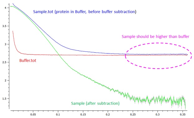
Fig 1. Confirmation of buffer subtraction. The .tot file is the averaged curve before the subtraction.
2. Guinier Plot
One can learn the overall
size of a protein by making a Guinier plot which gives an estimate of the radius
of gyration, Rg, and the forward scattered intensity, I(0). The latter is proportional
to the square of the molecular weight for a given number concentration.
These two quantities are useful in making sure that proteins are behaving well
under the x-ray beam. The plot is very simple: ln I(q) vs. q2.
It is critical that the plot be linear in the q range of q less than qmax=M/Rg,
where qmax is the upper q end-point of Guinier plot and M is typically 1.3 for globular protein.
If a straight line is not obtained, there are two possible scenarios:
downturn shape at low angle would be inter-particle repulsion of the sample.
Make sure that a consistent Rg value is obtained from all different sample concentrations and that all I(0) values are proportional to sample concentration. You might need to merge curves in case that concentration-dependence is observed (in this case you might need more comprehensive analyses, see below).
Programs used: SAXSPipe, Graphit (available at BL4-2), Primus, Primusqt and other mathematic/graphical software.

Fig 2. Guinier plot (Lysozyme)
3. Kratky Plot
The asymptotic behavior of intensity decay in the Porod regime following the Guinier region expresses the shape of your sample (Porod's law);
| Power law | Expected shape |
| q-4 | Spherical (~= very globular) |
| q-2 | Thin circular disk |
| q-2 | Gaussian chain (Random coil) |
| q-1 | Thin rod |
The Kratky plot, I(q)*q2 vs. q plot, is thus informative to check globularity and flexibility of your protein. In the case of well-folded globular protein, the Kratky plot will exhibit a "bell-shape" peak at low q and converges to the q axis at high q. The Kratky plot will not converge to the q axis if the protein has a pronounced flexibility. Proteins with multiple-domains could have additional peak(s) (or shoulders) at low q but the Kratky plot will still converge to the q axis at high q. If atomic or homology model is available, the Kratky plot should always be compared with data.
Make sure whether the peak position of all different concentration curves is identical. Strong interparticle effects, aggregation, multimerization and/or dissociation alter SAXS profile not only in low q but also higher q region (change the curvature in Porod region), suggesting that the shape of dominant sample are no more identical between different concentrations.
Programs used: Graphit (available at BL4-2), Primus, Primusqt and other mathematic/graphical software.
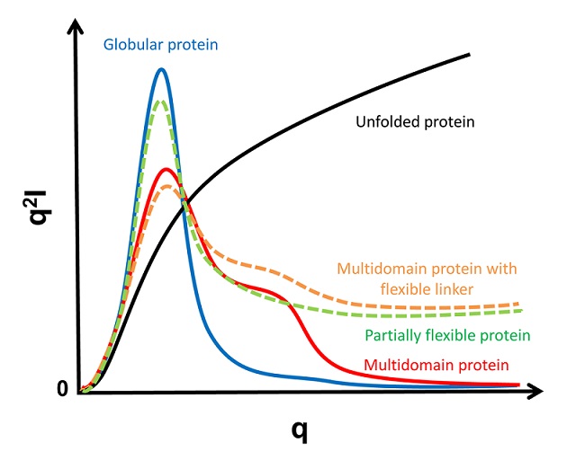
Fig 3. Schematic representation of typical Kratky plots. Curvature is depending on molecular shape, degree of flexibility, etc. Make sure that vertical axis (q2*I) is started from zero.
4. P(r) Function
The P(r) function, also known as Pair-wise distance distribution function or Distribution of inter-atomic distances, is usually obtained by taking an indirect Fourier transform of the scattering curve. It is important to have a good representation in the low angle region as well as at higher angles in order to reduce termination error in the Fourier transform. The useful parameter immediately obtained from the pair distribution function is the maximum dimension of the particle in solution, Dmax. P(r) drops to zero on the r axis where the maximum dimension is. The qmax should be greater than Pi/Dmax.
Real space Rg obtained by using the P(r) function should be consistent with reciprocal Rg obtained by using the Guinier Plot. Note that real space Rg is more accurate than reciprocal Rg and is less influenced by inter-particle interactions. If Kratky plot indicated flexibility, most programs for indirect Fourier transform are not applicable.
Programs used: Gnom, Primus and Primusqt (Gnom interface).

Fig 4. P(r) function.
5. Mw Estimation
There are several ways to estimate molecular weight (Mw) of your sample. Cross-validation between them is very important.
A. Water scattering
The program Graphit available at BL4-2 can estimate Mw based on water scattering data. Beamline staff provides you water scattering data at setup. See more details in J. Appl. Cryst. (2000). 33, 218-225.
B. Using protein standard
Take standard protein data that you know its Mw and concentration. Mw can be estimated as:
Mwexp / I(0)exp ≈ Mwstandard/I(0)standard
Standard protein, e.g. Lysozyme, RNaseA, etc, should be monodisperse, monomodal, globular protein in appropriate buffer. Please do not use BSA because it is generally mixture of monomer and dimer.
C. Porod volume
Mw ≈ Porod volume * 0.625
Gnom interface of the program Primusqt can straightforwardly estimate Porod volume concurrently with P(r). See Fig 3 above and more details in J. Appl. Cryst. (2012). 45, 342-350.
D. Dummy atoms
If you already did run ab-initio modeling like Dammin, Dammif and Gasbor, Mw could be estimated based on dummy atom volume:
Mw ≈ (Dammif or Dammin volume)/2
E. SAXS MoW
Useful JAVA applet at http://www.if.sc.usp.br/~saxs/
6. Merging Curves
Once zero concentration curve is successfully extrapolated (in other words, you confirmed that no more Rg change is detected at lower concentration curves), you could optionally combine the zero-concentration extrapolated curve with high concentration curve which possesses better signal in high q region. Before merging, make sure that the peak position of both Kratky plots is identical.
Programs used: Graphit (available at BL4-2), Primus, Primusqt and other mathematic/graphical software.
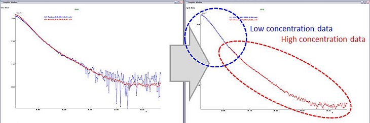
Fig 5. Merging curves.
7. Further Analysis
A variety of programs are available for further analysis. Note that most programs are designed for monomodal and monodisperse system without any flexibility. If data indicated flexibility, try the program for flexible system like EOM instead. Programs for multimodal system (e.g. mixture) are also developed recently.

