|
|
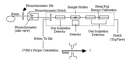
The basic components of a typical XAFS experiment are shown above (Figure 1). X-rays are produced in the source (bending magnets, wigglers, or undulators) and pass through an aperture before striking the monochromator. This aperture, a pair of slits, can be adjusted to control the size and energy resolution of the beam. Most monochromators at SSRL XAFS beam lines are double crystal designs. The first crystal of the pair can be detuned (rotated off of the Bragg condition) for precise alignment and for harmonic rejection. After entering the hutch, the beam passes through another defining aperture (Huber Ta slits). The beam passes through the gas in the gas ionization chambers, and its intensity is measured. These gas ionization chambers are typically used to measure the incident beam when filled with appropriate gas mixtures. Lytle or Germanium detectors are then used to measure fluorescent x-rays from the samples. The first step in an XAFS experiment is to align the beam line so that the most intense part of the beam is directed toward the hutch. The beam alignment procedure is as follow:
Gas Ionization Chambers
where Io is the photon flux of the incident beam, I1 is the photon flux of the transmitted beam, m is the absorption coefficient (cm2/g), r is the density of the gas (g/cc), and L is the length of the gas chamber (cm). By consideration of m of different gases and the desired percentage of transmission, an appropriate gas or gas mixture for each ion chamber can be chosen. Such an analysis is presented in Table 1. SSRL provides argon and nitrogen gases. Users can order other gases at their own expense.
Gain Settings For Ionization Chambers The voltage-to-frequency (V/F) converters are most linear between values of 0.5 V and 10 V. Hence, the gain for each Keithley amplifier for Io, I1, and I2 should be adjusted such that the V/F Converters give results in this range. The same also applies for Lytle detectors. Also, when working with Keithley amplifiers, it is essential to remember to set the suppression equal to the inverse of the gain. The Lytle detector, or the fluorescent ion
chamber detector, measures fluorescent x-ray emission. Fluorescence
arises from the de-excitation of electrons into the core hole produced
by x-ray photon absorption and is proportional to the probability of x-ray
photon absorption. Hence, fluorescence can be used to measure XAFS.
Fluorescence measurement has the greatest utility when using samples that
are dilute, have low K-edge energies, or are very small. Depending
upon the system being studied, it can be effective for concentrations down
to one part per million. Typically, the Lytle dectector is used for
samples having greater than 1000 parts per million of the metal ion of
interest. For more dilute samples, it is often necessary to use a
germanium detector. The advantages of the Lytle detector are its
much larger solid angle of acceptance and its ability to measure photons
at much higher count rates than germanium detectors. The use of germanium
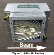
detectors are not covered in this document due to their complexity. When using a Lytle detector, most samples should be positioned such that the angle of incidence and exit are equal to 45o, which minimizes elastic scattering into the detector and maximizes the signal from the sample. The standard Lytle detector sample holder provides the 45o geometry. The sample should be mounted on the back of the holder. Additionally, one must insure that the Soller slits are positioned so that the fan of blades points in the direction of the x-ray beam (refer to Figure 2). For information on x-ray filters, refer to the section How to Select X-ray Filters. An important consideration for fluorescence measurements is what gas to use in the ion chamber of the Lytle detector. In general, it is desirable to use nitrogen for x-ray energies below 3 KeV, argon between 3-7 KeV, and krypton (or heavier gases) for energies above 7 KeV. For greater detail, refer to Table 2. Also, refer to the section Gas Ionization Chambers. When selecting gases for the Lytle detector, the theory is the same as for ion chambers, except that the Lytle chamber thickness is 3 cm and calculations should be based upon the energy of the fluorescence peak of the element of interest rather than the incident beam. The gas should absorb 90-95% of the radiation passing through the 3 cm distance of the Lytle chamber. Therefore, it is undesirable to use too heavy of a gas.
In a transmission measurement, the absorption spectrum of the sample is measured directly, as opposed to fluorescence or electron yield experiments. Key advantages to the transmission method are its simplicity and the absence of self absorption (nonlinear amplitude reduction effects), which is an inherent problem for fluorescence measurements of concentrated samples. Hence, transmission measurements are typically used for concentrated samples. Transmission data are plotted as Ln (Io/I1), which expresses absorption amplitude as a linear function of absorber concentration (and thickness). For transmission measurements, it is important that the gas ionization chambers be filled with appropriate gas mixtures (see Table 1 in Gas Ionization Chambers for useful gases and percentages of beam transmitted at various energy ranges). For a typical transmission measurement, the first gas ionization chamber should be filled with a gas mixture that will absorb about 22% of the incident beam. The second gas ionization chamber should then be filled with a gas mixture that will absorb as much of the remaining beam as possible in order to obtain the best counting statistics. The following procedure can be used as a guide to preparing transmission samples. It is based on the assumption that the absorption coefficient (mmetal) of the metal is much larger than the absorption coefficient of the matrix (mmatrix). If mmetal of the sample is comparable with mmatrix, the matrix will contribute substantially to background noise. For example, in a sample with two types of metal ions and both present in significant concentration (e.g. PbFe4O7), both metal ions will be dominant absorbers. Hence, the optimum sample mass may be different from the one obtained using the procedure that follows. The absorption by a sample with absorption coefficient ms and thickness L is related to the ratio of Io and I1 as exp (-msrL) = (I1/I0). Consideration of counting statistics in a transmission measurement has shown that the optimum product of msrL is 2.6, that is when the sample absorbs about 96% of the beam (Stern & Heald (1983), Brown, et. al.). However, the samples are often prepared in sample holders with standard sizes of 1 or 2 mm. Therefore, it is practical to achieve this optimum value by adjusting the sample's density instead of its thickness. In practice, best results have been obtained when the sample is prepared with a density that will absorb about 90% of the beam, that is, when msrx = 2.3. For a sample with known composition and density, ms can be calculated using the following summation:
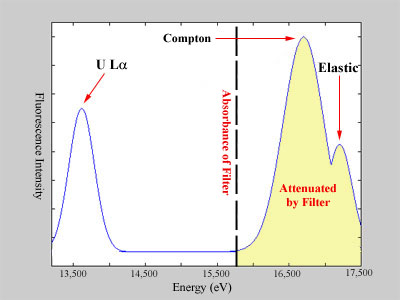
With the fluorescent method of detection one of the chief concerns is noise generated by the scattering of elastic plus Compton radiation by the sample. X-ray filters may be used to reduce the scattering radiation that enters the detector, making the choice of an x-ray filter an important consideration. When selecting a filter, the K-edge (or L-edge)
energy of the filter should be such that it absorbs much of the elastic
plus Compton radiation scattered by the sample, while simultaneously transmitting
the desired Ka radiation. For elements
from titanium (Ti) to ruthenium (Ru), it is preferable to select a x-ray
filter with element that has an atomic number of one less than the sample
that is, Z-1. Beyond Ru, either Z-1 or Z-2 elements may be used.
However, if the L-edge of a sample is be measured, it may be difficult
to find an element that satisfies the Z-1 or Z-2 condition for the filter.
For example, consider a uranium sample, whose La,
Compton, and elastic peaks are illustrated in Figure 4. The elements
satisfying the Z-1 or Z-2 condition are protactinium and thorium, both
of which are unavailable to use as filter elements. Therefore, the
periodic table must be searched to find an element that is both suitable
and available. That is, an element must be found with a K-edge energy
that will absorb the Compton and elastic radiation from the uranium sample.
A search reveals that strontium is an excellent candidate, with a K-edge
energy that will absorb much of the scattering radiation going towards
the detector.
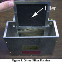
 The x-ray filter should be positioned so that it covers the Soller slits. One consideration when choosing a filter is its thickness. For dilute samples, it is often preferable to use a filter of 3 absorption lengths. For more concentrated samples, a filter of 6 absorption lengths probably will be optimal. However, each should be tried to ascertain which is best. Included is a table of selected elements to illustrate this (Table 3).
Resolution and Slit Dimensions The energy resolution of an XAFS beamline is controlled primarily by the monochromator and the vertical divergence of the beam. On many SSRL XAFS beam lines, the vertical beam divergence, described by the vertical opening angle of the beam, is defined by the vertical slits upstream of the monochromator. The vertical opening angle can be calculated trigonometrically from the source-slit distance and the vertical opening of the slits:
Energy calibration of monochromators
is needed because their calibration drifts over time due to missed steps
by the driving motor, computer problems, or changes in the synchrotron
orbits. Therefore, energy calibration should be checked frequently,
at least once a day after new fills. Reference materials (e.g.
metal foils that can be checked out from the SSRL store room) are used
as energy calibration for the position of the absorption edge. Absorption
edges for other elements should be found near their tabulated energies
after this calibration. The procedure for monochromator calibration
is as follow:
Before data collection may begin, the electronic
background signal should be measured. This is accomplished by taking
offsets. The computer will then be able to subtract the background
of electronic noise from the data during collection. The procedure
is both simple and brief:
Synchrotron radiation may simultaneously satisfy
the Bragg condition for multiple orders of diffraction (multiple n).
Bragg's Law is given by
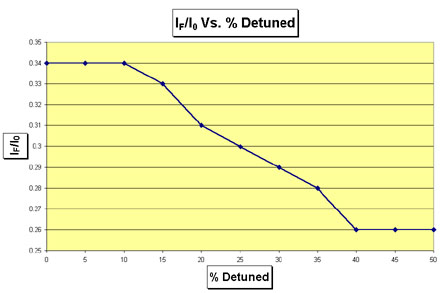
How to Determine The Proper Amount of Detuning To measure the amount of detuning required, a strong sample or foil of the element being investigated is placed in front of the Lytle detector. The monochromator is then set to an energy below the binding energy of the element. Thereby, most of the fluorescence emitted by the sample should result from harmonics in the beam, since they lie in higher energies than the fundamental. Create a table similar to Table 5 that has the following columns: percent detuned, I0, IF, and IF/I0. Make rows beginning with the monochromator fully tuned, 5% detuned, 10% detuned, and so on. Record the values for I0 and IF in the table. Then plot the ratio IF/I0 as a function of percent detuning. When the ratio of IF/I0 exhibits asymptotic behavior as it approaches a constant value, the desired amount of detuning has been achieved. As an example of the procedure for detuning, consider the actual detuning data collected for Uranium at beamline 4-3 of SSRL shown in Table 5 and Figure 5. The ratio IF/I0 becomes asymptotic at 40%. Therefore, as indicated in Table 5, the optimal detuning is 40%. However, the experimenter should verify that this level of detuning is actually necessary by comparing the noise levels of scans with different amounts od detuning.
Detuning should be checked often, and one should be mindful that the detuning may change as the temperature of the monochromator changes with variations in x-ray flux.
|
| Content Owner: John Bargar | Page Editor:
Ann Mueller |
Last Edited: 07 DEC 2004 |