| |

BL4-2 Home |
Data Processing Using SAPOKO
1) Detector response data Prepare an input file. A file detres.dat, for example, should look like: 1,10,1,1024,1,1,0,0,0,0.0,1.0e6,0,0,0
.9,0.
(empty
line)
Q01000.msk
(empty or anything)
Q01000.504
(detector response pattern)
Run sapoko from MS-DOS prompt:
Q01000.504 will be overwritten by the processed data. This file should have averaged intensities and standard deviation resulting from averaging. A log file should look like: DATE: 12-06-2002 TIME: 11:30
detector
response curves
Fidelity
treshold: .90000E+00 Min. relative error .00000E+00
No
detector response correction
Evaluated fidelity factors
1 .10000E+01 2 .10000E+01 3 .10000E+01 4 .10000E+01
5 .10000E+01 6 .10000E+01 7 .10000E+01 8 .10000E+01
9 .10000E+01 10 .10000E+01 11 .10000E+01 12 .10000E+01
13 .10000E+01 14 .10000E+01 15 .99988E+00
Number of frames averaged 15
Note that the all 15 individual curves (data frames) have high correlation so that all of them were averaged. 2) Calibration data Obtaining
s-axis file Run SAPOKO in the same way with a different input file. Here is an example: 1,10,1,1024,1,1,0,0,0,0.0,1.0e6,0,0,0
.9,0.
Q01000.504
Q01000.msk
(empty line) Q14000.504
Q15000.504
Output
file, cal.log:
DATE: 12-06-2002 TIME: 11:33
calibration
samples (cholesterol myristate, D=50.1 A)
Fidelity
treshold: .90000E+00 Min. relative error .00000E+00
Evaluated fidelity factors
1 .10000E+01 2 .10000E+01 3 .10000E+01
Number of frames averaged 3
Evaluated fidelity factors
1 .10000E+01 2 .10000E+01 3 .10000E+01
Number of frames averaged 3
FILE:
Q25001.504
Evaluated fidelity factors
1 .10000E+01 2 .10000E+01 3 .10000E+01
Run SAPOKO with a control file such as below. For detailed information about each line visit the SAPOKO manual at EMBL. 1,10,1,1024,1,1,1,0,0,0.0,1.0e6,0,0,0
.9,0.
Q01000.504
Q02000.msk
0,490,540,200,179,-0.01996,745,0.01996
Q02000.504
Q04000.504,Q03000.504,2.38
Q05000.504,Q03000.504,2.38
Q06000.504,Q08000.504,4.75
Q07000.504,Q08000.504,9.50
Q09000.504,Q08000.504,1.78
Q10000.504,Q08000.504,3.55
Q11000.504,Q08000.504,7.10
Q12000.504
Q13000.504
Q17000.504,Q16000.504,2.35
Q18000.504,Q16000.504,4.70
Q19000.504,Q16000.504,9.40
Q21000.504,Q20000.504,2.68
Q22000.504,Q20000.504,5.35
Q23000.504,Q20000.504,10.70
Q01000.504 is a detector response pattern you obtained above and Q02000.msk is a mask file for sample data processing. The fidelity threshold of 0.9 is used for averaging. The detector channels from 490 through 540 were used for Guinier plot. s (2pai*sin(theta)/lambda) values are specified by the locations of cholesterol myristate peaks: -1st order (s=-0.01996) at ch. 179 and 1st order (s=0.01996) at ch. 745. These values depend on actual experimental geometry and users must determine accordingly. B-SAXS/D staff can provide these parameters upon request.
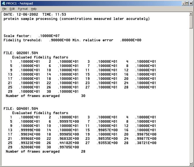
Top of log file proc1.log 4) Data statistics and quick evaluation of radii of gyration Determine the channel number that is the closest to the beam stop. Make it sure that scattering signal at this channel number is valid. Let's call it channel number X. This is typically several channels away from the edge of the beam stop. Let's call it X'. Try making Guinier plot in the channel range from X' through X'+Y, where Y is typically 20-50, depending on the actual Rg value. X and X+Y should be on the fifth line in
the control file, which also requires a couple of channel numbers where corresponding
s values are known. For instance, one can use (100) cholesterol myristate powder
diffraction peak at s=0.01996 Å-1. Round the cholesterol myristate peak
positions determined above to the nearest integers. The fifth line of the control
file should contain these numbers. In the example below(right, above???) ch.
AAA corresponds to this peak, and BBB is on the opposite side (-100) so that
the s value here is -0.01996. One can also use the second order peak at 0.03992
Å-1.
Bottom of log file prog1.log |
| webmaster (remove spaces in email address) | Last updated: December 9, 2005. |