Principal Component Analysis and Target Transformation Using EXAFSPAK: Notes For Version 0.1

Graham N. George and Ingrid J. Pickering

October 8, 2002

Stanford Synchrotron Radiation Laboratory

Summary of Analysis

Analysis is carried out using the EXAFSPAK programs, which are written by Graham George of SSRL.

1. Principal Component Analysis (PCA)

Analyze a series of unknown spectra to determine the number of principal components by:

generating the eigenvectors (principal components) and eigenvalues
plotting individual eigenvectors
testing elimination of eigenvectors on reconstruction of original spectra

2. Target Transformation (TARGET)

Test whether a given model spectra is a component of the series of unknown spectra.

3. Least Squares Refinement (DATFIT)

Fit the spectrum of an unknown to a linear combination of library spectra.

A "How-To" Guide

1. Principal Component Analysis (PCA)

Given a series of m related spectra of unknown composition, the program PCA is used to generate the eigenvectors (principal components) U and eigenvalues V. The m eigenvectors can be plotted. The elimination of eigenvectors with near-zero eigenvalues can be tested by graphically comparing each reconstructed spectrum with its original. Thus, a determination can be made about the number of principal components.

To start the PCA analysis, type:

PCA SAMP.HLD

SAMP.HLD is an ascii file containing the m filenames of the spectra of related unknowns. This can be created using a basic text editor, such as NOTEPAD. For example, SAMP.HLD might look like this:

SAMP1.EDG
SAMP2.EDG
SAMP3.EDG
SAMP4.EDG
SAMP5.EDG

After starting PCA, the following appears:

Principal Component Analysis.
Program PCA Version 0.1
Min, max eV to crop data [12599.2, 12748.5] : 12640 12710 (clip the energy range if desired)
Data files :
File 1 SAMP1.EDG
File 2 SAMP2.EDG
File 3 SAMP3.EDG
File 4 SAMP4.EDG
File 5 SAMP5.EDG
------------------------
Component   Eigenvalue
      1       35.9097
      2       3.43393
      3       2.86981
      4      0.880477
      5       1.32538
------------------------

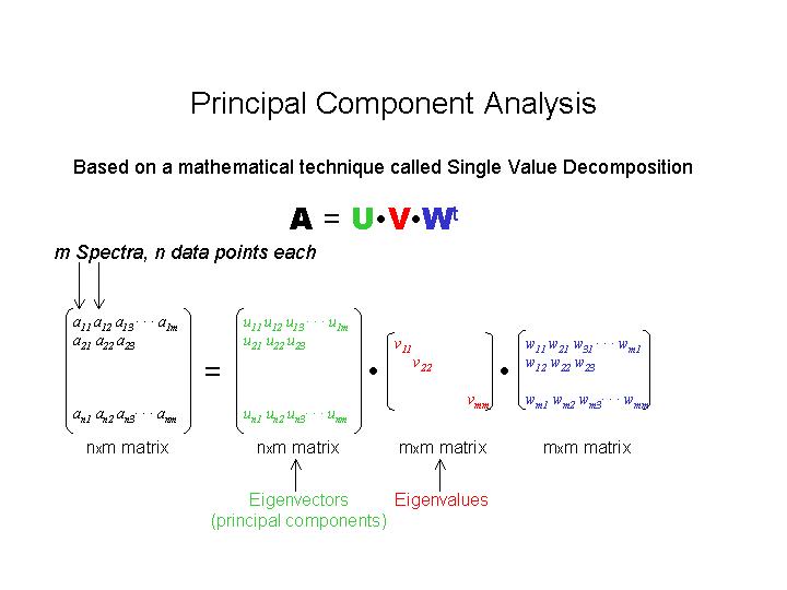
The eigenvalues of the m components are displayed. Some will be smaller than others; these are more likely to be able to be eliminated than the larger ones. However, it is difficult to predict which ones can be eliminated using this table alone. The next plot, of the individual eigenvectors, gives more information:

Press 1 to plot Eigenvectors :1
Enter GPLOT device number for plot [10] :
Enter route for plot [TT:] :

The m eigenvectors (principal components), scaled by their eigenvalues, will be displayed (U.V). Note that these principal components are not component spectra, but mathematical constructs. Some will show distinct features, while others may show essentially noise. These latter ones are the candidates for elimination. Based on the eigenvalues and the plots, use the next part of the program to test the elimination of eigenvalues.

Press 1 to plot Eigenvectors :
Press 1 to test Eigenvalues, 2 to quit :1
Enter Eigenvalue to eliminate [0] :4
------------------------
4 Eigenvalues
Total Residual : 0.3216760E-02
Component   Residual
      1      0.2194201E-02
      2      0.2202843E-04
      3      0.6603940E-03
      4      0.2082951E-03
      5      0.1318413E-03
------------------------

One eigenvalue is chosen to be eliminated - in this example #4 was chosen as it had the smallest eigenvalue and its plot looked like noise. After its elimination, the original spectra are reconstructed and the residual sum of squares is calculated for each spectra (see table above). If the eliminated eigenvector is not significant, then all the residuals will be low. However, the absolute value of the residuals will depend on the level of noise in the original spectra. The results can also be examined graphically:

Press 1 to plot :1
Enter Component to plot [1] :1
Enter GPLOT device number for plot [10] :
Enter route for plot [TT:] :

Component (original spectrum) 1 was chosen for this plot because it showed the largest residual, and therefore is most likely to show a real (i.e. greater than just the noise) deviation. All n components can be examined in this way. In this case of eigenvalue 4, the deviations are well within the level of the noise, and so this eigenvector is not contributing significantly. The elimination of the next component can then be tested; in our case #5 also is not significant, as judged by the reconstructed spectra. On testing the elimination of #3, however, the following is obtained:

Press 1 to plot Eigenvectors :
Press 1 to test Eigenvalues, 2 to quit :1
Enter Eigenvalue to eliminate [5] :3
------------------------
2 Eigenvalues
Total Residual : 0.4467924E-01
Component   Residual
      1      0.3871157E-02
      2      0.2383120E-01
      3      0.6740484E-03
      4      0.4575982E-02
      5      0.1172685E-01
------------------------

and the reconstructed spectra show significant deviations. Thus the elimination should be reversed:

Press 1 to plot :
Press 1 to undo elimination :1
Data files :
File 1 SAMP1.EDG
File 2 SAMP2.EDG
File 3 SAMP3.EDG
File 4 SAMP4.EDG
File 5 SAMP5.EDG
------------------------
Component   Eigenvalue
      1       35.9097
      2       3.43393
      3       2.86981
      4      0.000000E+00
      5      0.000000E+00
------------------------

and, having achieved a reasonable set of components, the program is exited:

Press 1 to plot Eigenvectors :
Press 1 to test Eigenvalues, 2 to quit :2

Thus, from PCA it can be concluded that three components are needed to fit this set of spectra. However, it gives no information about the spectral identity of those components. Note also that the elimination of eigenvalues is somewhat subjective. In the ideal case, with a perfect series of unknown spectra and no noise, the eigenvalues are rigorously zero. With the introduction of noise and other experimental uncertainties, these values are non-zero and whether or not to eliminate them becomes a more subjective question.

2. Target Transformation

Target transformation is used to test whether a standard or model spectrum is a component of the series of m unknown spectra. The program TARGET accomplishes this by using the file PCA.OUT, generated by PCA. Type the following:

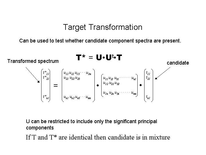
target model1.edg

and the model spectrum (T) will be graphically compared with its target transformation (T*). The graphical correspondence of the spectra, together with the residual value (displayed on the plot) can be used to test whether the spectrum is a component. Note that again this is a subjective test.

3. Least Squares Refinement

The program DATFIT carries out a least squares refinement of a series of model compounds to the spectrum of an unknown. Model spectra can be identified using TARGET and then used in DATFIT. If PCA shows that x (x < m) principal components are needed and TARGET identifies x components, then these can be used in the analysis.

Please refer to the documentation on Edge Analysis for more information on DATFIT.

Acknowledgments

SSRL is funded by the Department of Energy, Offices of Basic Energy Sciences and Biological and Environmental Research; the National Institutes of Health, National Center for Research Resources, Biomedical Technology Program, and the National Institute of General Medical Sciences.