In order to do this, we need to record the spectra of a series of standard compounds which are candidates for what is in the unknown. These should be as similar as possible to what is there; for example, differences are found between crystalline solid and aqueous solution of the same compound, and between different allotropes of an element. Hence, the reliability of the results will strongly reflect the appropriateness of the standards used. Care should also be taken that the standards are collected under the same conditions as the sample, e.g. same energy resolution and conditions of calibration, as these may bias the results.
Having acquired a library of standard spectra, selected spectra are used in a least-squares fitting procedure to simulate the spectrum of the unknown. Once a "good" fit is achieved, the percentage contribution of a standard spectrum to the fit is considered to be equivalent to the percentage of the element present in that form.
The method works best for a small number of chemical components whose spectra are substantially different. It cannot be used to distinguish or quantitate between very similar spectra. Although it can work on relatively low elemental abundances, it cannot detect a trace of one chemical form of the element in presence of a large excess of another form of the same element.
Suppose we have five sweeps of data, collected using a multi-element detector:
MYSAMPLE_037.001To examine individual fluorescence (FF) channels in a single sweep of 30-element data (NUM=7-19 for 13-element detector):
MYSAMPLE_037.002
MYSAMPLE_037.003
MYSAMPLE_038.001
MYSAMPLE_038.002
MVIEW/NUM=10-39/DEN=4 MYSAMPLE_037.001For sum of fluorescence channels in all sweeps of 30-element data (NUM=7-19 for 13-element detector):
MVIEW/NUM=10-39/DEN=4/SUM MYSAMPLE_037.00*,MYSAMPLE_038.00*
MCALIB/ELEM=AS/OUT=MYSAMPLE.CAL MYSAMPLE_037.001By default the program uses log(I1/I2), and the smoothed first derivative. It also assumes a K-edge ( /EDGE=L3 will use the L3 edge). You will see a plot of the foil spectrum, the smoothed first derivative, and vertical lines marking peaks in the latter. If needed, use the left/right arrows to move the highlighted peak, but usually the strongest inflection is also the desired first inflection (an exception: for Mo K-edge, the strongest is the second, so need to move to the first). When the desired peak is highlighted, hit return to exit and write the calibration point to the specified file, in this example MYSAMPLE.CAL. Then repeat with each of the sweeps for this sample:
MCALIB/ELEM=AS/OUT=MYSAMPLE.CAL MYSAMPLE_037.002When done, MYSAMPLE.CAL will have a list of filenames, each energy calibration point, as well as the element and tabulated calibration point.
MCALIB/ELEM=AS/OUT=MYSAMPLE.CAL MYSAMPLE_037.003
MCALIB/ELEM=AS/OUT=MYSAMPLE.CAL MYSAMPLE_038.001
MCALIB/ELEM=AS/OUT=MYSAMPLE.CAL MYSAMPLE_038.002
MAVE/OUT=MYSAMPLE.AVE/MCALIB=MYSAMPLE.CAL* If the calibration points found are very similar, answer N. This will average all the sweeps and shift by the mean calibration difference. As this does not require interpolation of the data, this is preferable. However, if the calibration point is varying significantly (e.g. >0.3 eV for As or Se), averaging the data this way would broaden the spectral features. Therefore, in this case shift the spectra individually.5 Files found :
1 MYSAMPLE_037.001
2 MYSAMPLE_037.002
3 MYSAMPLE_037.003
4 MYSAMPLE_038.001
5 MYSAMPLE_038.002Do you want to remove files from this list? [y/n] [N] : (use this to remove a file if needed)
Do you want to change file weights? [y/n] [N] :
Enter array position for eV [3] :
Enter array position for rtc [1] :
Enter array position range for numerator [7, 19] : 10,39 (7,19 for 13-element; 10,39 for 30-element)
Enter array position range for denominator [4, 4] :
Do you want to take logs? [y/n] [N] :
Do you want to change array position weights? [y/n] [N] : (use to remove a channel from all sweeps)
Do you want to perform deadtime corrections? [y/n] [Y] :n
Statistical weights :
Enter 1 to calculate, 2 to use weights from file, 3 for unit weights [2] :
Do you want to exclude specific array positions? [y/n] [N] :(use to exclude channels in single sweeps)
Recalibration ...
Do you want to shift individual spectra? [y/n] [N] : (see * below)
Enter apparent eV0, true eV0 [11865.5, 11867.0] :
Enter d-space, steps per degree [1.92016, 100000.] :
Enter Za, E0 [33.0000, 11885.0] :
My sample info
File MYSAMPLE_037.001
...
PROCESS MYSAMPLEThe program automatically looks for the .AVE file.
Press 1 to subtract baseline file :(a) The eV(high) value should be below the onset of the edge. If the edge is strong, this value may need to be decreased from the default value.
Press 1 to plot baseline subtraction :
Press 1 to subtract pre-edge :1
Press 1 for polynomial pre-edge fit, 2 for Gaussian, 3 for erf function :2
Enter eV(low), eV(high) [0.0, 11840.0] :,11820 (a)
Enter energy eV for middle of SCA window [10543.0] :
Enter window width, detector resoln. (eV) [750.000, 250.000] : ,700 (b)
Enter scaling factors a, b (y=a*y+b) [5.62004, .290140] :
Press 1 to plot pre-edge result :1
To "try again" with different numbers, type Ctrl-Z and choose the baseline/pre-edge option (2) from the main menu.
For very weak samples (the scatter tail is by far the dominant feature, spectrum appears very noisy), the background is much more difficult tofit. Some suggestions to make it work:
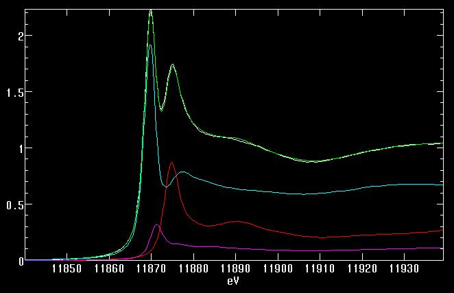
Press 1 to subtract Spline :1If the background has been well computed, then the spline (green) and the Victoreen (red) should overlay (for high energies, see above). If not, use Ctrl-Z to return to the background subtraction and tweak the "detector resoln." (increase if spline is sloping down too much to high energy, and vice versa). However, only change if the pre-edge remains visually flat.
Do you wish to reset to defaults? [y/n] [Y] : (2nd or more type Y here)
Enter Spline eV(low) & eV(high) [11885.0, 12033.0] :
Enter order of Spline & No. of ranges [4, 3] :2 2 (use 2,2 for short edge range)
Enter k-weighting for spline [4] :
Enter 1 to use Victoreen [1] :
Enter 1 for k-spaced spline points [0] :
Enter 1 Spline Points
Spline Point 0 [11885.0] :
Spline Point 1 [11959.0] :
Spline Point 2 [12033.0] :
Enter symbol for element [AS] :
Enter edge (K, L1,..) [K] :
Enter Victoreen Coefficients Cvic,Dvic [262.000, 95.4000] :
Enter Edge jump u0 for ratio (0 = auto) [0.0] :
Enter eV to calc. u0 [11905.0] : (the spline value at this eV is used to normalize)
Using calculated value for u0 ( 0.22633 )
final falloff was 0.97
Press 1 to plot spline removal :
Press 1 to plot spline removal + Victoreen :1
The .EDG file is an ASCII file which can be plotted using the EXAFSPAK
program MULDAT or alternatively exported to another graph-plotting program.
e.g. filename: DATFIT_AS.HLDLaunch DATFIT using
ARSENATE-AQ.EDG
ARSENITE-AQ.EDG
ASGS3.EDG
AS-ELEM.EDG
DATFIT DATFIT_AS.HLDand select 1 to read in data.
Enter name of file to be fitted [ ] :MYSAMPLE.EDGIt is a good idea to keep the fit range ("Clip data") fairly broad. For Se use 12600,12750.
Enter col. nos for x,y [1, 2] :
Clip data - enter min. and max. x-values [2460.00, 2490.00] : 11840,11940
Enter parameter filename [ ] :MYSAMPLE.PAR
Enter No. of components for fit [4] :3
Component 1 - Select file by number [1] :
Enter col. nos for x,y [1, 2] :
...
Component 1 - Enter initial fraction, eV shift [0.0, 0.0] : 0.2E.s.d. - the estimated standard deviation derived from the diagonal elements of the variance-covariance matrix. Often we quote three times the e.s.d., which is the 99% confidence limit. Note that this is a measure of the precision of the parameter in the fit but not its accuracy. The accuracy of the result will be somewhat poorer and depends, in particular, on the appropriateness of the standards and the quality of the data.
Enter 1 to fix fraction, eV shift [0, 1] :
...
Enter max. no of iterations [5000] :Fit complete
( Info = 6 )
File MYSAMPLE.EDG Edge
Energy range (eV) : 11840.0 - 11940.0
# Fraction e.s.d. eV-shift e.s.d. i i File
1 0.257040 0.996237E-03 0.000000E+00 0.000000E+00 0 1 [-]ARSENATE-AQ.EDG
2 0.101991 0.183439E-02 0.000000E+00 0.000000E+00 0 1 [-]ARSENITE-AQ.EDG
3 0.637315 0.165220E-02 0.000000E+00 0.000000E+00 0 1 [-]ASGS3.EDGNo. of function evals : 15
No. of variables : 3
No. of data points : 335
Residual : 0.117783E-03
Total : 0.996346
D ratio : 30.5793
Residual - the mean sum of squares of the differences between observed and calculated normalized intensities, S(Iobs-Icalc)2/N, where Iobsand Icalc are the observed and calculated normalized intensities, respectively, and the summation is over N data points. The smaller the residual the better the fit for a given unknown spectrum. Note that noise contributes to the residual so a noisy spectrum will always have a bigger residual than a clean one.
Total - the sum of the fractions, which ideally should be unity. Deviation from this indicates either that the spectra have not been normalized in the same way or that the standards used in the fit are not properly representative of the components of the sample.
D ratio - do not use.
Some suggestions:
Output - option 4. Two files can be written:
Enter filename for output [ ] : MYSAMPLE.OUTThe parameter file holds information on the component number, fractions and eV shifts (if any) for use in future fits.
Enter parameter filename [MYSAMPLE.PAR] :
The output file is a text file of various spectra. This can be used, together with the original .EDG file, to produce a custom plot in MULDAT. Alternatively, these files can be exported to another graph-plotting program. For a 3-component fit the columns are as follows:
- 1 - energy
- 2 - calculated fit spectrum
- 3-5 - spectra of components 1-3, with eV shifts (if any) applied but not scaled. (i.e. to generate a fit plot, scale these components by the respective fractions obtained).
- 6 - residual spectrum
| Program | Fluorescence using Lytle detector | Transmittance | Reference foil transmittance |
| MVIEW | MVIEW/NUM=7/DEN=4 | MVIEW/NUM=4/DEN=5/TAKE | MVIEW/NUM=5/DEN=6/TAKE |
| MAVE | numerator: [7,7] | numerator: [4,4]
denominator: [5,5] takelogs: Y |
numerator: [5,5]
denominator: [6,6] takelogs: Y |
| PROCESS | Polynomial background, order -1 or -2*. | Polynomial background, order -1 or -2*. | Polynomial background, order -1 or -2*. |
*Adjust range and order to make a flat pre-edge and a coincident spline.
MVIEW options |
Default |
Comments |
| /help | none | Displays all options for this program. |
Data Manipulation: |
||
| /numerator=<arg> | /num=7-19 | Specify array of numerator channels. Can use range (e.g. 10-39), or
pick (e.g. 12;13;14-17)
See table below for channel positions for different detector configurations. |
| /denominator=<arg> | /den=4 | Specify denominator channel(s). Generally den=4 for I0. Use den=1 to divide by count time only. |
| /takelog | do not take log | Take the logarithm of the specified (num/den). |
| /sumdata | plot individual traces | Sum all specified numerator channels. |
| /normalize | do not normalize | Normalize to the maximum intensity in each trace. |
| /abscissa=<arg> | /abs=3 | Specify abscissa (x-axis) channel. Energy is abs=3. Use
abs=index to plot vs. point number. |
Plot Style: |
||
| /xminimum=<arg>
/xmaximum=<arg> |
extent of data | Specify plot range for x-axis. |
| /yminimum=<arg>
/ymaximum=<arg> |
extent of data | Specify plot range for y-axis. |
| /cursors | no cursors | Invoke cursors to find position, mark or zoom (cursors can also be called by typing c with plot displayed) |
| /highlight | no highlight | Highlights (in yellow) single channel while remainder are in blue. Press space bar to cycle between channels. |
| /colours=<arg> | default colour map | Specify colours for plotting. |
| /points[=<arg>] | no points | Specify style of plot points. (0=single pixel, 1=squares, 2=triangles, etc) |
| /noline | plot line | Do not plot line (useful if plotting points). |
Output: |
||
| /route=<arg> | /route=TT: | Specify plot to file (route=filename) or to screen (default, route=TT:). |
| /device=<arg> | /device=10 | Specify plot device type (10=x-windows, 2=regis, 8=postscript, 9=encapsulated postscript). |
| /xwindows=<arg> | /xwindows=on | Specify whether x-windows is used or not. |
| /write[=<arg>] | do not write | After plotting to screen, output to ascii file(s). |
Keystroke files: |
||
| /logfile[=<arg>] | none | Record keystroke file (default logfile is MVIEW.LOG) |
| /recover[=<arg>] | none | Replay keystroke file (default logfile is MVIEW.LOG). |
| /dumb | none | No output to screen while replaying keystroke file (useful for file generation alone). |
| Nature of problem | Description | Possible fix at beamline | Fix during data analysis |
| Monochromator crystal glitch | Sharp peaks or dips, in all channels and all sweeps, caused by Bragg diffraction of the monochromator "stealing" intensity from main beam | Try detuning more | None |
| Windowing problem with single channel | Single channel output has no edge jump (all sweeps) while others do. Window for this channel is not correct. | Check windowing | Exclude channel |
| Electronic problem with single channel | Single channel is zero or has abnormally high noise (some or all sweeps) for a variety of possible reasons. | Ask for help | Exclude channel |
| Sample diffraction peaks | Spikes or dips in individual channels, reproducible sweep to sweep. ICR channels have many extraneous peaks. This can occur if a composite sample has crystalline particles (e.g. a soil) or if a solution sample is frozen too slowly and forms ice crystals. | If frozen solution, flash freeze or use glassing agent (e.g. glycerol). If peaks not too large, reduce total count rate. | If visible in FF channels, exclude channel |
| Sample changing in beam | Systematic change in edge shape from sweep to sweep, most likely caused by beam damage (or possibly reaction with air, etc.) | To minimize photon damage, lower temperature (use lHe cryostat), and/or scan more quickly | Use only 1st sweep (but may have already changed) |
| Beam motion | Excursion in all channels of single sweep. Also present in I0. | None (restart sweep) | Exclude sweep |
| Short sweep | MVIEW plot all bunched up in one corner. Run was terminated in middle of sweep. | None (don't stop run in middle of sweep) | Exclude short sweep from MVIEW plot |
| Countrates too high | ICR maximum countrate above ~150k cps (for dilute) or 100k cps (for concentrated). Spectral features may appear "squashed" due to deadtiming. | Move detector back | Check transmittance data |
| Sample too concentrated | Self-absorption means that fluorescence signal from a concentrated sample is distorted, irrespective of sample. | If this is a standard solution, check the dilution. 5-10 mM is a good range for fluorescence. | Transmittance data may be usable |
MVIEW/NUM=10-12;14;16;17-19/DEN=4 MYSAMPLE_037.001For all individual fluorescence channels in all sweeps:
MVIEW/NUM=10-39/DEN=4 MYSAMPLE_037.00*,MYSAMPLE_038.00*To examine individual total incoming countrate (ICR) channels in a single sweep of 30-element data (NUM=20-32 for 13-element detector), useful if looking for sample diffraction:
MVIEW/NUM=40-69/DEN=4 MYSAMPLE_037.001To check actual countrates (ICRs) for a single sweep of 30-element data (NUM=20-32 for 13-element detector):
MVIEW/NUM=40-69/DEN=1 MYSAMPLE_037.001To plot incident intensity I0 for all sweeps:
MVIEW/NUM=4/DEN=1 MYSAMPLE_037.00*